Guide
How to choose the right Solver.
This section explains the trade off between the three solvers available in fastFM. The following applies for both classification and regression tasks.
import fastFM.mcmc
- (+) smallest number of hyper parameter
- (+) automatic regularization
- (-) predictions need to be calculated at training time
Note: The predict method of the mcmc model returns predictions based on only the last draw of the model parameters. This evaluation is fast but usually of low quality. Don’t use mcmc if you need fast predictions!
import fastFM.als
- (+) fast predictions
- (+) less hyper parameter then SGD
- (-) regularization must be specified
import fastFM.sgd
- (+) fast predictions
- (+) can iterate over large datasets (split and iterate over junks using warm start)
- (-) regularization must be specified
- (-) highest number of hyper parameter (requires, step_size)
Learning Curves
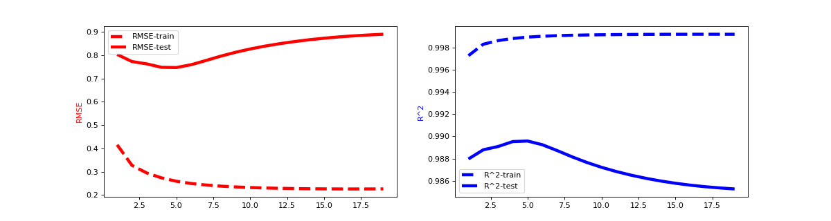
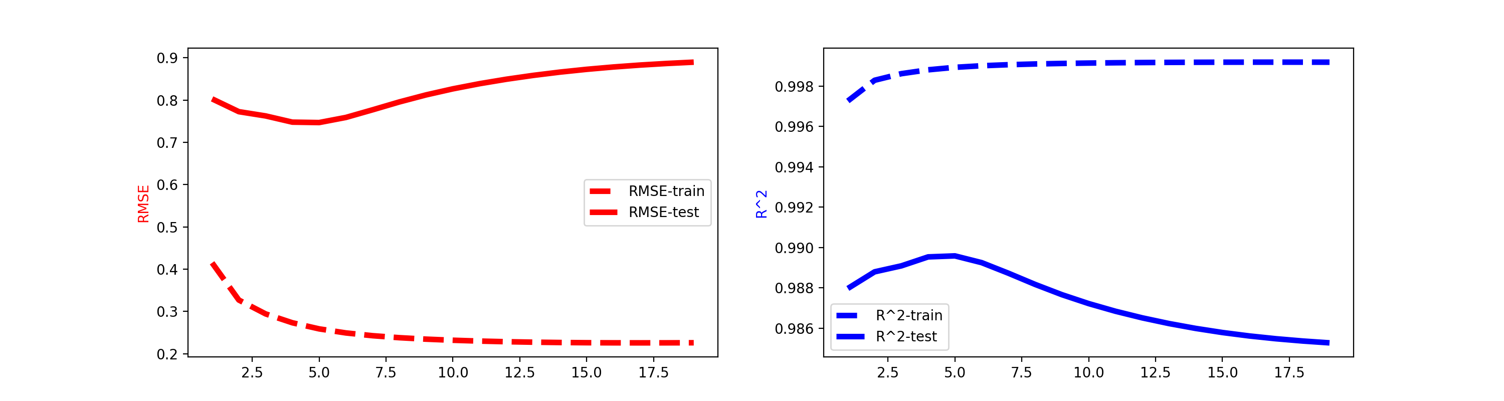
Learning curves are an important tool to understand the model behavior and enable us to use techniques such as early stopping to avoid over fitting. We can warm_start every fastFM model which allows us to calculate custom statistics during the model fitting process efficiently. The following example uses RMSE and R^2 to demonstrate how we can monitor model performance on train and test set efficiently. Please note that we can replace them with any metric we want.
from fastFM import als
from fastFM.datasets import make_user_item_regression
from sklearn.metrics import mean_squared_error, r2_score
import numpy as np

X, y, coef = make_user_item_regression(label_stdev=.4)
from sklearn.model_selection import train_test_split
X_train, X_test, y_train, y_test = train_test_split(
    X, y, test_size=0.33, random_state=42)

n_iter = 20
step_size = 1
l2_reg_w = 0
l2_reg_V = 0

fm = als.FMRegression(n_iter=0, l2_reg_w=0.1, l2_reg_V=0.1, rank=4)
# Allocates and initalizes the model parameter.
fm.fit(X_train, y_train)

rmse_train = []
rmse_test = []
r2_score_train = []
r2_score_test = []

for i in range(1, n_iter):
    fm.fit(X_train, y_train, n_more_iter=step_size)
    y_pred = fm.predict(X_test)

    rmse_train.append(np.sqrt(mean_squared_error(fm.predict(X_train), y_train)))
    rmse_test.append(np.sqrt(mean_squared_error(fm.predict(X_test), y_test)))

    r2_score_train.append(r2_score(fm.predict(X_train), y_train))
    r2_score_test.append(r2_score(fm.predict(X_test), y_test))


from matplotlib import pyplot as plt
fig, axes = plt.subplots(ncols=2, figsize=(15, 4))

x = np.arange(1, n_iter) * step_size
with plt.style.context('fivethirtyeight'):
    axes[0].plot(x, rmse_train, label='RMSE-train', color='r', ls="--")
    axes[0].plot(x, rmse_test, label='RMSE-test', color='r')
    axes[1].plot(x, r2_score_train, label='R^2-train', color='b', ls="--")
    axes[1].plot(x, r2_score_test, label='R^2-test', color='b')
axes[0].set_ylabel('RMSE', color='r')
axes[1].set_ylabel('R^2', color='b')
axes[0].legend()
axes[1].legend()
(Source code, png, hires.png, pdf)

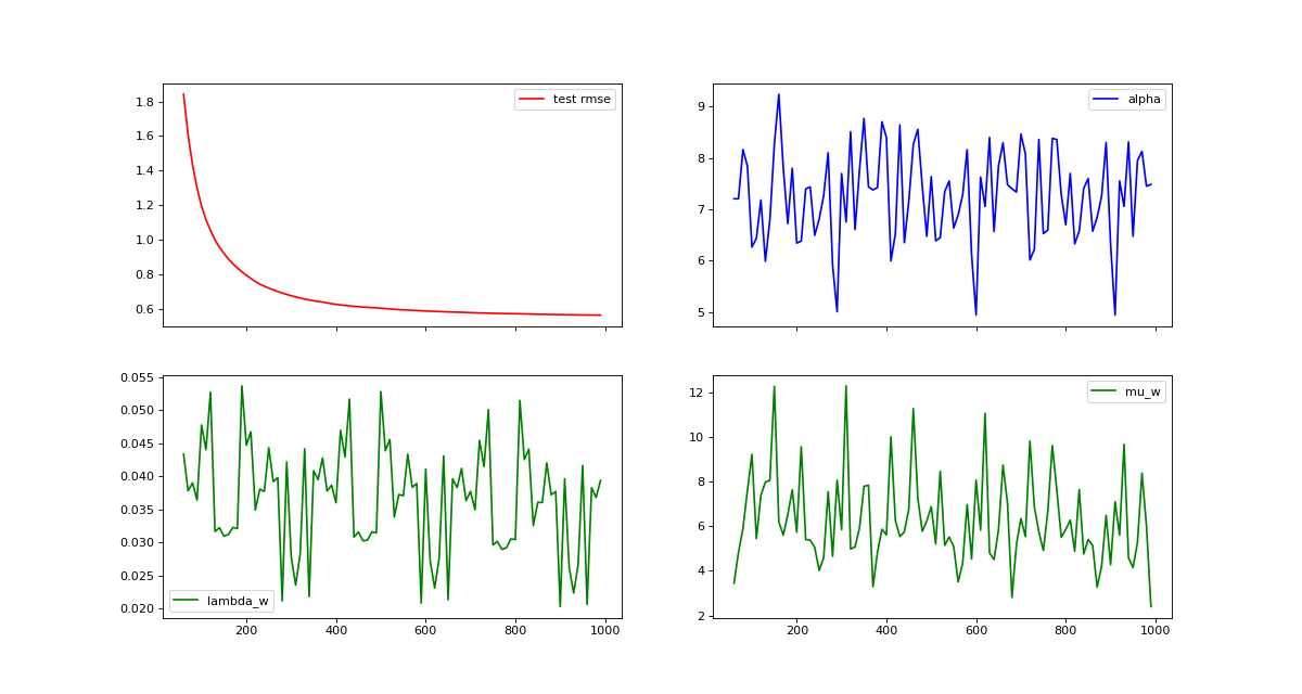
Visualizing MCMC Traces
Our MCMC implementation samples model and hyper parameter at every iteration and calculates a running mean of the predictions. MCMC traces are an important tool for evaluating convergence and mixing behavior MCMC chains. The following example demonstrates how to calculate statistics for predictions, hyper parameter and model parameter efficiently using the warm_start option.
import numpy as np
from sklearn.metrics import mean_squared_error
from sklearn.model_selection import train_test_split

from fastFM.datasets import make_user_item_regression
from fastFM import mcmc

n_iter = 100
step_size = 10
seed = 123
rank = 3

X, y, coef = make_user_item_regression(label_stdev=.4)
X_train, X_test, y_train, y_test = train_test_split(
    X, y, test_size=0.33)

fm = mcmc.FMRegression(n_iter=0, rank=rank, random_state=seed)
# Allocates and initalizes the model and hyper parameter.
fm.fit_predict(X_train, y_train, X_test)

rmse_test = []
rmse_new = []
hyper_param = np.zeros((n_iter -1, 3 + 2 * rank), dtype=np.float64)
for nr, i in enumerate(range(1, n_iter)):
    fm.random_state = i * seed
    y_pred = fm.fit_predict(X_train, y_train, X_test, n_more_iter=step_size)
    rmse_test.append(np.sqrt(mean_squared_error(y_pred, y_test)))
    hyper_param[nr, :] = fm.hyper_param_

values = np.arange(1, n_iter)
x = values * step_size
burn_in = 5
x = x[burn_in:]

from matplotlib import pyplot as plt
fig, axes = plt.subplots(nrows=2, ncols=2, sharex=True, figsize=(15, 8))

axes[0, 0].plot(x, rmse_test[burn_in:], label='test rmse', color="r")
axes[0, 0].legend()
axes[0, 1].plot(x, hyper_param[burn_in:,0], label='alpha', color="b")
axes[0, 1].legend()
axes[1, 0].plot(x, hyper_param[burn_in:,1], label='lambda_w', color="g")
axes[1, 0].legend()
axes[1, 1].plot(x, hyper_param[burn_in:,3], label='mu_w', color="g")
axes[1, 1].legend()
(Source code, png, hires.png, pdf)
